Forecasting Project
Yeongjun Oh
4/20/2020
Through my academic and professional experience as a Marketing Analyst Intern, I have learned how to analyze data and gain a passion for analytics, especially forecasting. The law and order that governs how this world operates can be calculated and challenged through Data Analytics. For businesses, it could mean that calculating consumer patterns based on seasonality and, thus, can estimate future customer behaviors will bring efficient allocation of resources. In this project, I’m going to forecast the CPI, the Consumer Price Index. The Consumer Price Index is inflation in the United States, representing changes in the general price level and cost of living.
Although I used CPI for this model, these methods are applicable and versatile for a number of variations. For instance, these skills allow one to forecast sales, consumer behavior research, or even the impact of a recession on sales.
My primary objective is to exemplify how great R can be used as an analytics and data visualization tool. I hope this encourages others to use R to make pretty and interactive graphs.
Libaries & Data Visualization
In R, there are a lot of libraries that can be used at your disposal. I’ve used the following libraries for this project.
library(vars)
library(dplyr)
library(ggplot2)
library(forecast)
library(tseries)
library(readr)
library(DT)
library(dplyr)
library(latticeExtra)
library(xts)
library(dygraphs)
library(tidyverse)
library(lubridate)
This is how I imported the data. Data
GithubData <- "https://raw.githubusercontent.com/monetarist/monetarist.github.io/master/Final_Exam_Data.csv"
FinalData <- read_csv(GithubData)
Followings are the explanations for the variables.
GDPC1 is the Real Gross Domestic Product quarterly data.
FGOVTR is the Federal Government Tax Receipts quarterly data.
FFR is the Federal Funds Rate quarterly data.
NETEXP is the Net Export quarterly data.
MDOAH is the Mortgage Debt Outstanding quarterly data.
CPI is the Comsumers Price Index quarterly data.
DGS10 is the 10-Year Treasury Constant Maturity Rate quarterly data.
unrate is the unemployment rate quarterly data.
IP is the industrial Production quarterly data.
PD is the Public Debt quarterly data.
This is the Data Table.
This is a time series graph of Real GDP and CPI. Since these two variables are correlated, I have used these two variables to build a VAR model. See VAR model & IRF tab for more info!
The size of the data points show the magnitude of the public debt (Bigger sizes show the bigger public debts). The color scale represents Industrial Production (The light blue indicates bigger Industrial Production index). Y-axis is the Federal Government Tax Receipts and the X-axis is the CPI. By using an interactive graph, one can look at the correlation between 4 variables.
It’s clear that the Government Tax Receipts, Industrial Production and Public debt are all positively correlated with CPI. However, it’s not wise to conclude the correlation equals causation. Further analysis is required to check the true correlation between these varibles since all variables are positively correlated. To mitigate these issues, a few forecasting models have been designed to control the effects of other varibles into forecasting. See Principal Component tab for more info.
Decomposition
Decomposition of CPI data. The time series model can be decomposed into 3 components: trend, seasonality, and remainder. The trend is the rate of change of the data, which shows the longterm progression of the series. The seasonality is a change in the series/data in fixed intervals with a similar magnitude. The remainder is the random fluctuation in the data.
These are the decomposition of the CPI data. The seasonal indices indicate that there’s small or no seasonality in the data.
Decompose_CPI = stl(CPI, s.window = "per")
autoplot(Decompose_CPI)
Seasonality of the CPIDSeason_CPI = seasonal(Decompose_CPI)
DSeason_CPI## Qtr1 Qtr2 Qtr3 Qtr4
## 1966 -0.14222086 -0.12779233 0.19909442 0.07091882
## 1967 -0.14222086 -0.12779233 0.19909442 0.07091882
## 1968 -0.14222086 -0.12779233 0.19909442 0.07091882
## 1969 -0.14222086 -0.12779233 0.19909442 0.07091882
## 1970 -0.14222086 -0.12779233 0.19909442 0.07091882
## 1971 -0.14222086 -0.12779233 0.19909442 0.07091882
## 1972 -0.14222086 -0.12779233 0.19909442 0.07091882
## 1973 -0.14222086 -0.12779233 0.19909442 0.07091882
## 1974 -0.14222086 -0.12779233 0.19909442 0.07091882
## 1975 -0.14222086 -0.12779233 0.19909442 0.07091882
## 1976 -0.14222086 -0.12779233 0.19909442 0.07091882
## 1977 -0.14222086 -0.12779233 0.19909442 0.07091882
## 1978 -0.14222086 -0.12779233 0.19909442 0.07091882
## 1979 -0.14222086 -0.12779233 0.19909442 0.07091882
## 1980 -0.14222086 -0.12779233 0.19909442 0.07091882
## 1981 -0.14222086 -0.12779233 0.19909442 0.07091882
## 1982 -0.14222086 -0.12779233 0.19909442 0.07091882
## 1983 -0.14222086 -0.12779233 0.19909442 0.07091882
## 1984 -0.14222086 -0.12779233 0.19909442 0.07091882
## 1985 -0.14222086 -0.12779233 0.19909442 0.07091882
## 1986 -0.14222086 -0.12779233 0.19909442 0.07091882
## 1987 -0.14222086 -0.12779233 0.19909442 0.07091882
## 1988 -0.14222086 -0.12779233 0.19909442 0.07091882
## 1989 -0.14222086 -0.12779233 0.19909442 0.07091882
## 1990 -0.14222086 -0.12779233 0.19909442 0.07091882
## 1991 -0.14222086 -0.12779233 0.19909442 0.07091882
## 1992 -0.14222086 -0.12779233 0.19909442 0.07091882
## 1993 -0.14222086 -0.12779233 0.19909442 0.07091882
## 1994 -0.14222086 -0.12779233 0.19909442 0.07091882
## 1995 -0.14222086 -0.12779233 0.19909442 0.07091882
## 1996 -0.14222086 -0.12779233 0.19909442 0.07091882
## 1997 -0.14222086 -0.12779233 0.19909442 0.07091882
## 1998 -0.14222086 -0.12779233 0.19909442 0.07091882
## 1999 -0.14222086 -0.12779233 0.19909442 0.07091882
## 2000 -0.14222086 -0.12779233 0.19909442 0.07091882
## 2001 -0.14222086 -0.12779233 0.19909442 0.07091882
## 2002 -0.14222086 -0.12779233 0.19909442 0.07091882
## 2003 -0.14222086 -0.12779233 0.19909442 0.07091882
## 2004 -0.14222086 -0.12779233 0.19909442 0.07091882
## 2005 -0.14222086 -0.12779233 0.19909442 0.07091882
## 2006 -0.14222086 -0.12779233 0.19909442 0.07091882
## 2007 -0.14222086 -0.12779233 0.19909442 0.07091882
## 2008 -0.14222086 -0.12779233 0.19909442 0.07091882
## 2009 -0.14222086 -0.12779233 0.19909442 0.07091882
## 2010 -0.14222086 -0.12779233 0.19909442 0.07091882
## 2011 -0.14222086 -0.12779233 0.19909442 0.07091882
## 2012 -0.14222086 -0.12779233 0.19909442 0.07091882
## 2013 -0.14222086 -0.12779233 0.19909442 0.07091882
## 2014 -0.14222086 -0.12779233 0.19909442 0.07091882
## 2015 -0.14222086 -0.12779233 0.19909442 0.07091882
## 2016 -0.14222086 -0.12779233 0.19909442 0.07091882
## 2017 -0.14222086 -0.12779233 0.19909442 0.07091882
## 2018 -0.14222086 -0.12779233 0.19909442 0.07091882autoplot(DSeason_CPI)+ ylab("Seasonality")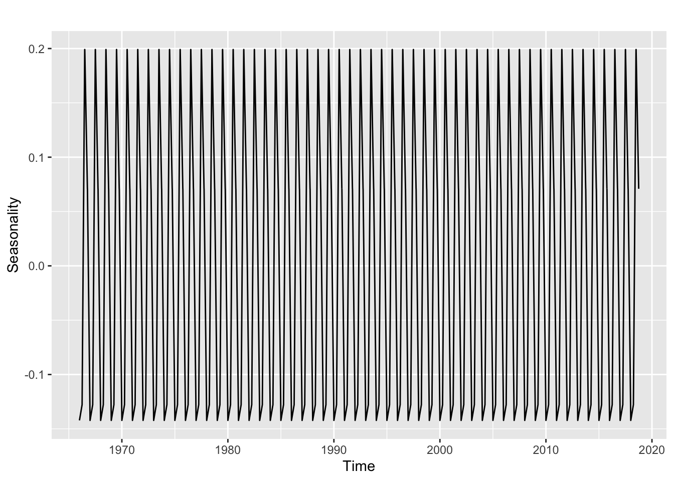
By analyzing the seasonal index and the graph, it’s clear that CPI data has seasonality. This is how you interpret the Seasonality Index. If the seasonal index is 0.01, then the CPI (or your variable) will be 1% lower than the trend. Due to seasonality, the CPI will decline 14 and 12 percent from the trend in the first and second quarters, respectively. Furthermore, CPI will likely to increase 19 and 7 percent more than the trend due to seasonality during the first and second quarters, respectively. As the CPI can change more than 10% due to seasonality, it’s clear that there’s contributing seasonality.
This is deseasonalized plot of the CPI
Deseasonal_CPI = seasadj(Decompose_CPI)
autoplot(Deseasonal_CPI)+ ylab("Deseasonal CPI")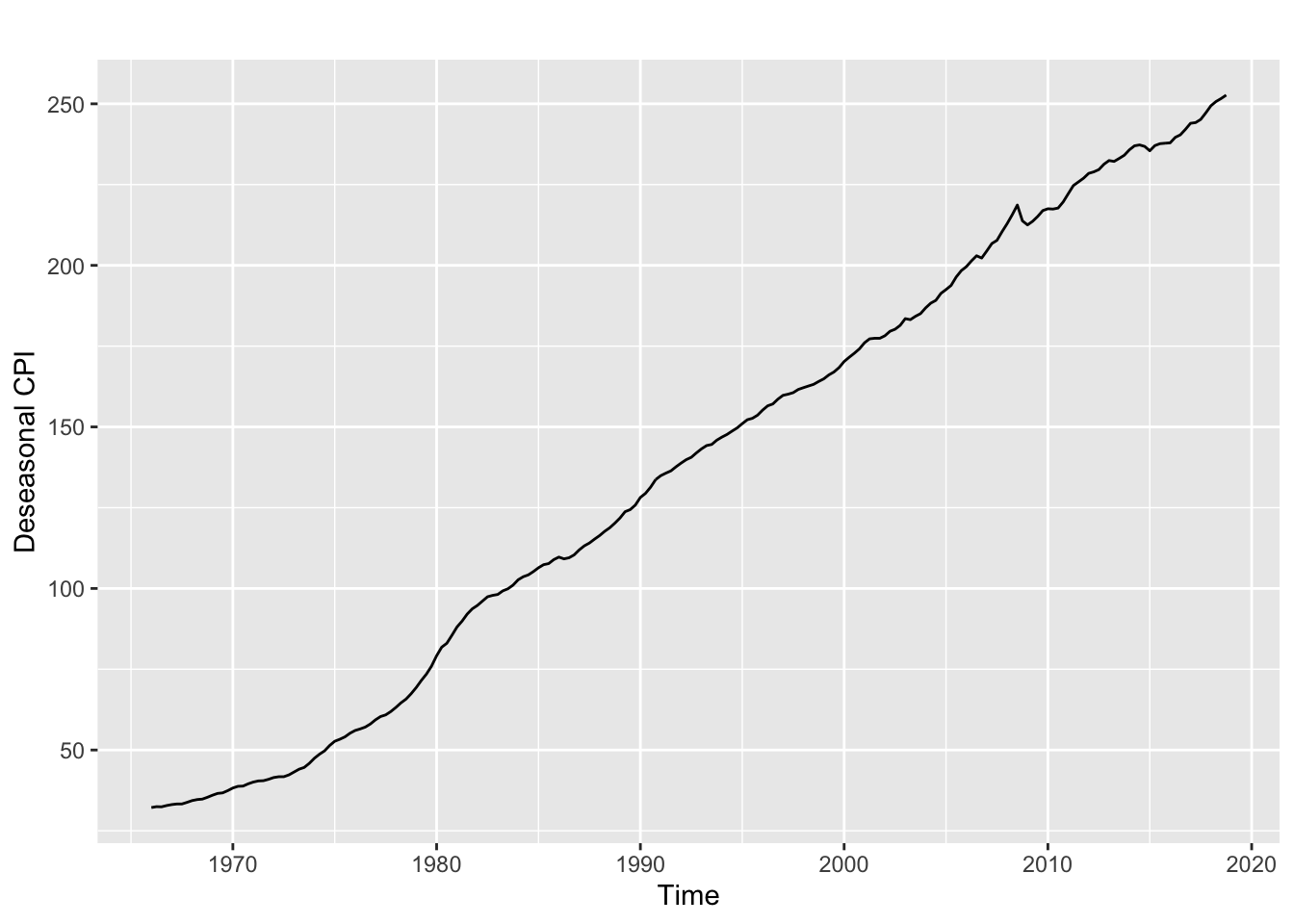
The deseasonalized plot focuses on the trend and avoids confusion from seasonal fluctuation.
ARIMA Model
ARIMA is a time series model that looks at autoregressive (AR), moving average (MA), and order of integration (I). There’s a lot of detail that I can’t explain in this project. More information is available in the link.
Using auto.ARIMA to find appropriate ARIMA model.The auto.arima function lets the R choose an ARIMA model. Since R automatically chose a SARIMA model, it’s an indicator that the seasonality exists.
CPI_ARIMA = auto.arima(CPI)
checkresiduals(CPI_ARIMA)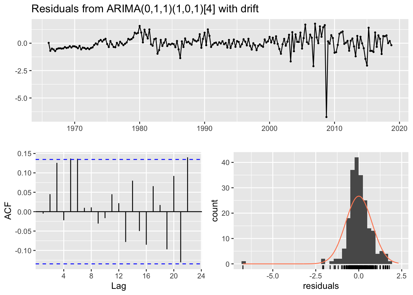
##
##  Ljung-Box test
##
## data:  Residuals from ARIMA(0,1,1)(1,0,1)[4] with drift
## Q* = 12.248, df = 4, p-value = 0.0156
##
## Model df: 4.   Total lags used: 8
The first step of forecasting is to check the model’s accuracy. One can do this by checking the residual, which is what differentiates between model (what we expected) and what’s observed (the data). When one is analyzing the data, one should prefer to get white noise, which indicates that the model is unbiased if the White Noise is from a forecasting model or regression. Another way to interpret the white noise is the Breusch Godfrey test. The Breusch-Godfrey test indicates whether the null hypothesis is rejected or not (the null hypotensis indicates that residuals are not correlated) through white noise residuals. This is the residual plot, ACF, and the histogram of the residuals. The researchers want white noise.
In this specific model, the residual plot indicates that the mean of the residuals is 0. The ACF of the residuals is below the confidence interval. The histogram of the residuals is under the normal distribution. From the following evidences, one can conclude that the residuals are white noise.
The Ljung-Box indicates that the model was looking at 4 seasonal observations (4 quarters).
Forecasting with ARIMA model selected by auto.ARIMAWith the auto.arima function, the R will automatically choose a ARIMA model that maximizes the accuracy (by minimizing AIC).
CPI_ARIMA_Forecast = forecast(CPI_ARIMA, h =3)
CPI_ARIMA_Forecast
## Point Forecast Lo 80 Hi 80 Lo 95 Hi 95
## 2019 Q1 253.7208 252.7230 254.7187 252.1948 255.2469
## 2019 Q2 254.7666 253.0451 256.4882 252.1338 257.3995
## 2019 Q3 255.8209 253.6002 258.0417 252.4246 259.2173autoplot(CPI_ARIMA_Forecast)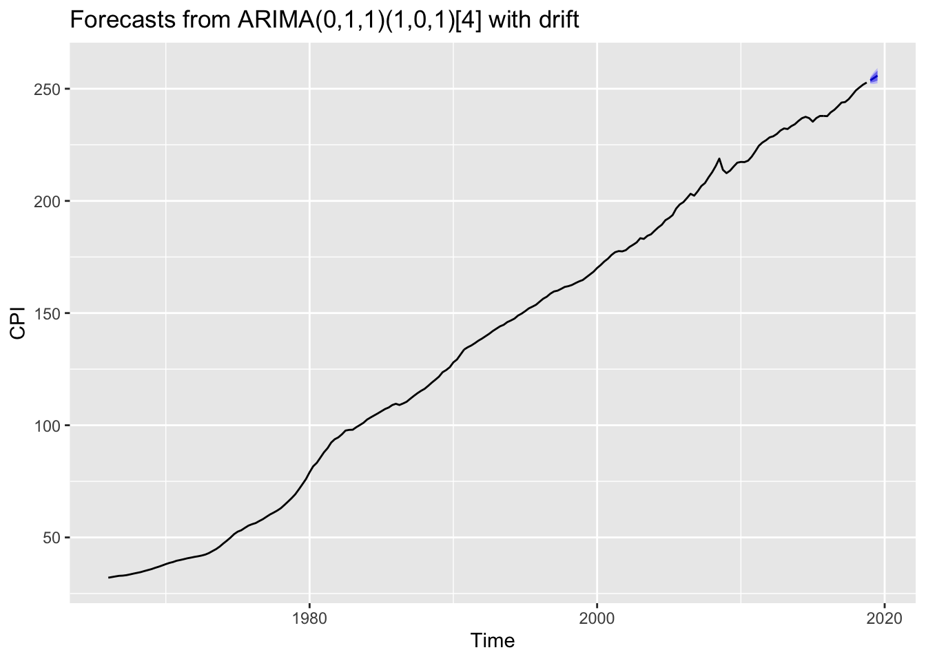
With the auto-selected “auto.arima” model, the model is predicting the CPI in 2019 Q1, Q2, and Q3 is going to be 253.72, 254.76, and 255.82 , respectively.
Customizing ARIMA fucntionOne can customize the ARIMA function by changing the code. In this model, I’ve selected ARIMA (0,1,1) without a drift model (basic exponential smoothing model).
Final_Model1 = Arima(CPI, order = c(1,1,1), include.drift = FALSE)
Question2B = forecast(Final_Model1, h =3)
Question2B
## Point Forecast Lo 80 Hi 80 Lo 95 Hi 95
## 2019 Q1 253.9222 252.8873 254.9572 252.3395 255.5050
## 2019 Q2 255.0719 253.4618 256.6819 252.6095 257.5342
## 2019 Q3 256.2080 254.0549 258.3611 252.9152 259.5008Unlike the " auto.arima " function, the (0,1,1) ARIMA model (basic exponential smoothing model) with a drift have identical forecast, initally. However, the difference between both models becomes bigger as the time progresses.
autoplot(Question2B)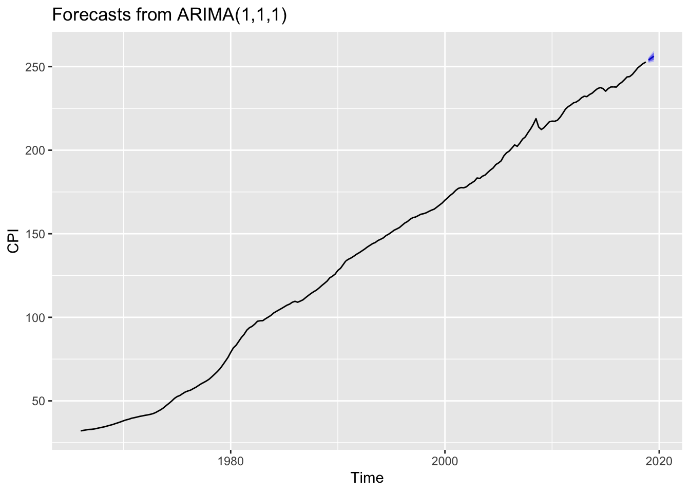
checkresiduals(Final_Model1)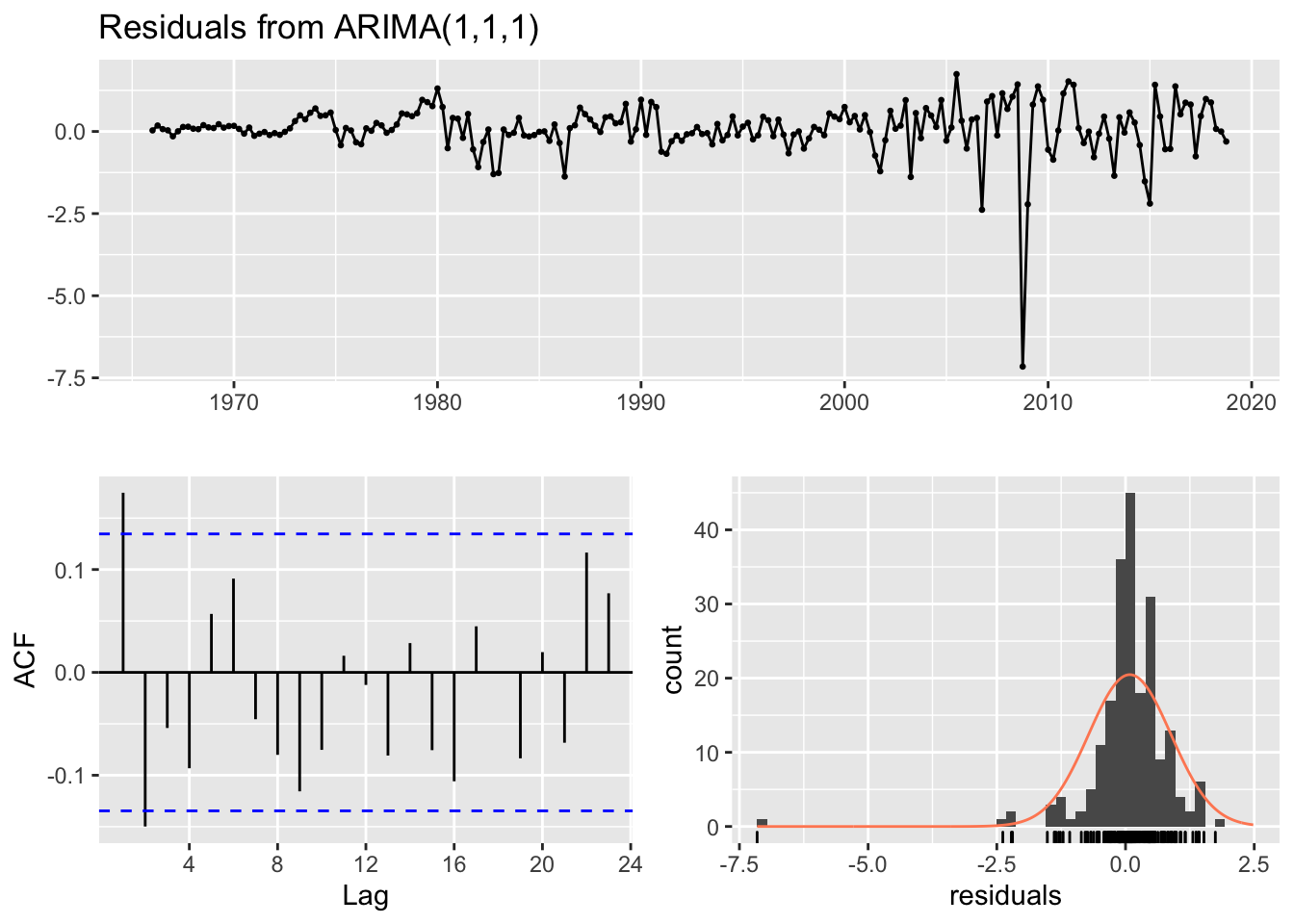
##
##  Ljung-Box test
##
## data:  Residuals from ARIMA(1,1,1)
## Q* = 18.36, df = 6, p-value = 0.005393
##
## Model df: 2.   Total lags used: 8
These are the residual plot, ACF, and the histogram of the residuals for the ARIMA (0,1,1) model. It’s hard to conclude that the mean of the residuals is zero from the residual plot. The ACF of the residuals is above the confidence interval. The histogram of the residuals is under the normal distribution. From the following evidence, residuals are not white noise. Therefore, the residual of the model is biased.
Fitting a linear trend model with an ARIMA error structure to the CPI dataThe ARIMA error models include autocorrelated errors in the model. In laymen’s terms, it’s a regression model that incorporates changes in time when considering the correlation between variables. In typical regression models, the error is considered white noise and ignored. The linear trend model with the ARIMA error structure helps the selection of predictors. To find a predictor from the variables, One needs to use an ARIMA error structure model with all other variables and choose the variable with the lowest AIC. However, for simplicity, I’ll demonstrate with a simple trend equation (it’s essentially counting).
By adding an xreg option into the " auto.arima " function, one can make the ARIMA error structure.
 TrendCPI = c(1:length(CPI))
 fit = auto.arima(CPI, xreg = TrendCPI)
 fcast = forecast(fit, xreg= c(213,214,215))
 #fcast
 fit
## Series: CPI
## Regression with ARIMA(1,0,1) errors
##
## Coefficients:
## ar1 ma1 intercept xreg
## 0.9806 0.4106 24.7775 1.0698
## s.e. 0.0134 0.0667 5.5103 0.0388
##
## sigma^2 estimated as 0.6009: log likelihood=-246.87
## AIC=503.74 AICc=504.04 BIC=520.53The model produces the following regression model.
\(y_{t} = 24.775 + 1.0698 x_{t} +n_{t}\)
\(n_{t} = 0.9806n_{t-1} +\epsilon + 0.4106 \epsilon\)
\(\epsilon\) ~ \((0,0.6009)\)
Where \(n_{t}\) is an ARIMA (1,0,1) error.
If we forecast based on this model, the following is going to be the forecast.
fcast## Point Forecast Lo 80 Hi 80 Lo 95 Hi 95
## 2019 Q1 253.7250 252.7316 254.7185 252.2057 255.2444
## 2019 Q2 254.7740 253.0719 256.4761 252.1709 257.3771
## 2019 Q3 255.8234 253.6477 257.9991 252.4959 259.1509The auto.ARIMA function predicted that the CPI is going to be 253.7208 in 2019 Q1. The ARIMA error model has a very close forecast of 253.7250.
Regression Forecasting
This a standard Regression Forecasting model with seasonality. (Regression Forecasting Model is similar to FORECAST.ETS.SEASONALITY function in Excel) The regression model provides the accuracy of the seasonality.
CPItrendRegression = tslm(CPI ~ trend+season)
 summary(CPItrendRegression)
##
## Call:
## tslm(formula = CPI ~ trend + season)
##
## Residuals:
## Min 1Q Median 3Q Max
## -9.4006 -2.5182 0.6727 2.7547 13.5339
##
## Coefficients:
## Estimate Std. Error t value Pr(>|t|)
## (Intercept) 17.389368 0.791456 21.971 <2e-16 ***
## trend 1.123358 0.004908 228.869 <2e-16 ***
## season2 -0.058276 0.849478 -0.069 0.945
## season3 -0.022457 0.849521 -0.026 0.979
## season4 -0.210368 0.849591 -0.248 0.805
## ---
## Signif. codes: 0 '***' 0.001 '**' 0.01 '*' 0.05 '.' 0.1 ' ' 1
##
## Residual standard error: 4.373 on 207 degrees of freedom
## Multiple R-squared: 0.9961, Adjusted R-squared: 0.996
## F-statistic: 1.31e+04 on 4 and 207 DF, p-value: < 2.2e-16According to the Regression Model, Compared to the first quarter, season 2 and 3 is expected to be slightly lower than the season1. The low coefficient for season 2 and 3 indicate the seasonality is weak or doesn’t exist. The high p-value for the seasons indicates that there is no seasonality. However, there is a strong positive trend for CPI.
Forecasting with Regression model CPIRegressionForecast = forecast(CPItrendRegression, h =3)
CPIRegressionForecast## Point Forecast Lo 80 Hi 80 Lo 95 Hi 95
## 2019 Q1 256.6645 250.9490 262.3801 247.9000 265.4291
## 2019 Q2 257.7296 252.0140 263.4452 248.9650 266.4942
## 2019 Q3 258.8888 253.1732 264.6044 250.1242 267.6534Comparing accuracy of Regression & ARIMA error structure modelaccuracy(CPIRegressionForecast, d =1, D =0)## ME RMSE MAE MPE MAPE MASE ACF1
## Training set -9.723207e-16 4.321008 3.361012 0.1059919 4.877736 2.925139 0.9570962accuracy(fcast, d =1 , D=0)## ME RMSE MAE MPE MAPE MASE ACF1
## Training set -0.03736094 0.7678488 0.4978913 -0.16188 0.4998526 0.4333221 -0.004795397The first line is the accuracy of the Regression Model and the second line is the accuracy for the ARIMA error structure model. One can use the accuracy results such as ME, MAE and MAPE to compare the accuracy of the models, but I’m going to use RMSE. The RMSE stands for Root Mean Square Error. The lower number is an indication of an accurate model.
I used d =1 & D =0 to the accuracy function because it’s the default. The default will be used throughout the project for consistency. The RMSE for the " auto.arima" model was lower. Thus I’ve concluded that the " auto.arima " is more accurate than the Simple Regression Model.
VAR Model & IRF
In typical OLS, the model assumes that (example of OLS is y = f(x) ) x is not dependant. VAR model is a time series model that assumes that all variables are treated as an endogenous variable. In laymen term, it checks the dependencies of all variables.
So I’m going to choose a variable that’s highly correlated to the CPI and fit a Vector Autoregressive model using p = 1 (only one lag). To choose the variable, I printed a correlation matrix.
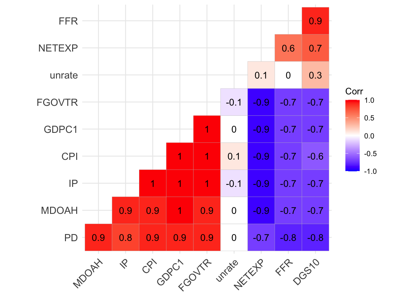
The CPI & Real Gross Domestic Product has a strong correlation. So I’m going to use CPI & Real Gross Domestic Product to build a Vector Autoregressive model.
Modeling a Vector Autoregressive modelRGDP = ts(FinalData$GDPC1, frequency = 4, start = c(1966,1,1))
options(scipen = 999)
VARselect(CPI, RGDP, lag.max = 4, type = 'const')## $selection
## AIC(n) HQ(n) SC(n) FPE(n)
## 1 1 1 1
##
## $criteria
## 1 2 3 4
## AIC(n) -Inf -Inf -Inf -Inf
## HQ(n) -Inf -Inf -Inf -Inf
## SC(n) -Inf -Inf -Inf -Inf
## FPE(n) 0 0 0 0var = VAR(cbind(CPI, RGDP), p =2, type = 'const')
summary(var$varresult$CPI)##
## Call:
## lm(formula = y ~ -1 + ., data = datamat)
##
## Residuals:
## Min 1Q Median 3Q Max
## -6.7989 -0.3240 -0.0311 0.3594 1.7561
##
## Coefficients:
## Estimate Std. Error t value Pr(>|t|)
## CPI.l1 1.3532865 0.0654832 20.666 < 0.0000000000000002 ***
## RGDP.l1 0.0007009 0.0007498 0.935 0.3510
## CPI.l2 -0.3539239 0.0657727 -5.381 0.000000201 ***
## RGDP.l2 -0.0006836 0.0007515 -0.910 0.3640
## const 0.5383545 0.2156578 2.496 0.0133 *
## ---
## Signif. codes: 0 '***' 0.001 '**' 0.01 '*' 0.05 '.' 0.1 ' ' 1
##
## Residual standard error: 0.7815 on 205 degrees of freedom
## Multiple R-squared: 0.9999, Adjusted R-squared: 0.9999
## F-statistic: 4.026e+05 on 4 and 205 DF, p-value: < 0.00000000000000022So the VARselect function provides me with the optimal lag length for the model. All criteria are suggesting 1 lag. But I’m going to go with 2 lags.
The responses up to 3 periods for both variables due to a one-unit shock in each variable
Impulse ResponseI’m going to model an impulse Response to see how exogenous events can impact both variables. One way of understanding impulse Response is what’s the impact of GDP if there’s a shock in CPI. First, I’m going to but a shock in GDP and observe CPI’s response.
 var1=irf(x=var, impulse="RGDP", response = "CPI", boot=TRUE, ortho = FALSE,n.ahead = 3,runs = 1000)
 var1
##
## Impulse response coefficients
## $RGDP
## CPI
## [1,] 0.0000000000
## [2,] 0.0007008689
## [3,] 0.0012178495
## [4,] 0.0015021497
##
##
## Lower Band, CI= 0.95
## $RGDP
## CPI
## [1,] 0.0000000000
## [2,] -0.0007154798
## [3,] -0.0010766558
## [4,] -0.0010142103
##
##
## Upper Band, CI= 0.95
## $RGDP
## CPI
## [1,] 0.000000000
## [2,] 0.002334511
## [3,] 0.004217409
## [4,] 0.005222146Shock in the GDP will have little or no impact to the CPI. Largely CPI stayed stationary.
1 unit shock for CPI var2=irf(x=var, impulse="CPI", response = "RGDP", boot=TRUE, ortho = FALSE, runs = 100)
plot(var2)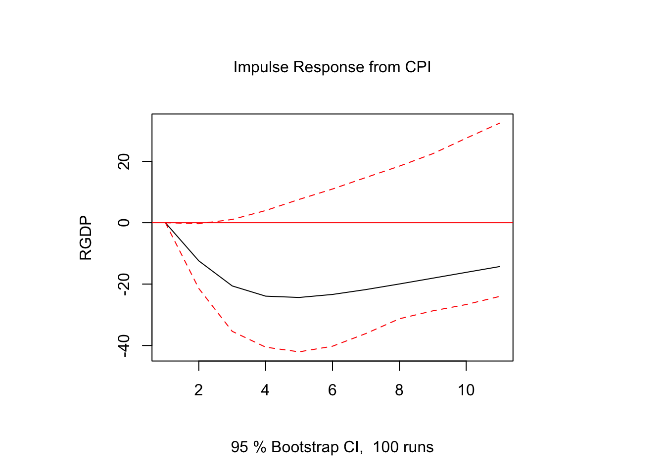
However, CPI’s shock will impact the GDP. By analyzing the results in economic thoeries, it’s very logical. The Real GDP excludes the inflation (such as CPI) from it’s calculation. Therefore, a shock in the Real GDP won’t impact the CPI as real GDP is independent of price changes. However, the shock in the inflation can impact the Real GDP. For instance, huge hyper inflation or deflation will impact the real economy becuase of unstable prices.
3 Point Forecast for CPI & GDP from the Vector Autoregressive ModelUsing AIC criteria to determine the optimal lags in the VAR and generating forecast values for the assigned variable up to 3 periods forward.
fvar = forecast(var, h=3)
fvar$forecast$CPI
## Point Forecast Lo 80 Hi 80 Lo 95 Hi 95
## 2019 Q1 253.8238 252.8223 254.8253 252.2921 255.3555
## 2019 Q2 254.9527 253.2581 256.6472 252.3610 257.5443
## 2019 Q3 256.1096 253.8515 258.3677 252.6561 259.5630VAR Modelvar4 = VAR(y=cbind(CPI, RGDP), p =1, type = 'const')
fvar2 = forecast(var4, h =3)
fvar2$model##
## VAR Estimation Results:
## =======================
##
## Estimated coefficients for equation CPI:
## ========================================
## Call:
## CPI = CPI.l1 + RGDP.l1 + const
##
## CPI.l1 RGDP.l1 const
## 1.00206479446 -0.00001474409 0.91930933597
##
##
## Estimated coefficients for equation RGDP:
## =========================================
## Call:
## RGDP = CPI.l1 + RGDP.l1 + const
##
## CPI.l1 RGDP.l1 const
## 0.5308657 0.9953667 44.4094228The var model above is a slightly different one as the p = 1. (p is for Lag)One can retrieve the A matrix & \(\epsilon_{t}\). The Impulse Response Functions are produced by putting impact into A matrix.
\[ Y_{t}= \left(\begin{array}{cc} 1.00206479446 & -0.00001474409\\ 0.5308657 & 0.9953667 \end{array}\right) \left(\begin{array}{cc} Y_{1,t-1} \\ Y_{2,t-1} \end{array}\right) + \left(\begin{array}{cc} 0.91930933597 \\ 44.4094228 \end{array}\right) \]
Auto.ARMA Model & VAR model accuracy comparisonFor consistency, accuracy setting is at d =1 and D = 0. The following is the accuracy of the VAR model.
accuracy(fvar, d=1, D=0)## ME RMSE MAE MPE MAPE MASE ACF1
## CPI Training set -0.000000000000000676728 0.77214 0.4828257 -0.059786044 0.4327868 0.4202104 0.01620901
## RGDP Training set 0.000000000000025988008 67.19114 49.7865194 -0.008608207 0.5271594 0.5883980 -0.08499249This is the result of the ARIMA model results inaccuracy.
accuracy(CPI_ARIMA_Forecast)## ME RMSE MAE MPE MAPE MASE ACF1
## Training set 0.003907738 0.7693755 0.4884155 -0.08925105 0.4603931 0.1145306 -0.004847103RMSE for the Var model was higher, thus ARIMA has higher accuracy.
Principal Component
The principal component can be used to reduce the number of regressors (variables) in the model. But PC allows keeping most of the info as possible while reducing the regressors. If you want to learn about the statistical theory behind the PC, check out the link.
Adding a principal component with all of the variablespca = prcomp(cbind(RGDP,FGOVTR,FFR,NETEXP,MDOAH,DGS10,unrate, IP, PD))
summary(pca)## Importance of components:
## PC1 PC2 PC3 PC4 PC5 PC6 PC7 PC8 PC9
## Standard deviation 5267381 1084 107.4 85.63 6.723 2.803 1.941 1.342 0.5789
## Proportion of Variance 1 0 0.0 0.00 0.000 0.000 0.000 0.000 0.0000
## Cumulative Proportion 1 1 1.0 1.00 1.000 1.000 1.000 1.000 1.0000plot(pca$x[,1])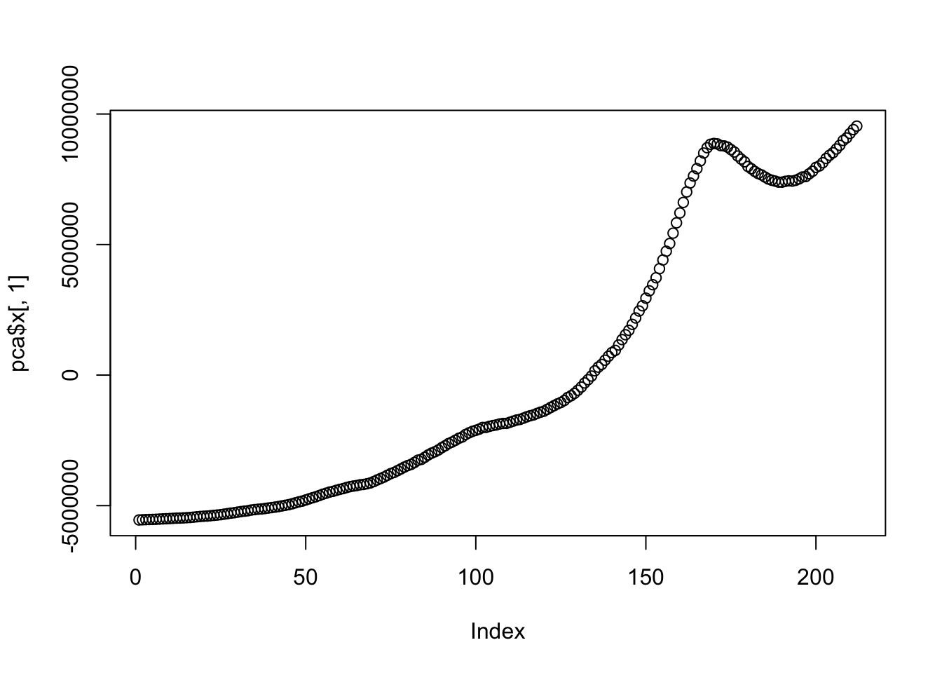
pc = ts(pca$x[,1], frequency = 4, start = c(1966,1,1))
summary(pc)
## Min. 1st Qu. Median Mean 3rd Qu. Max.
## -5548587 -4624375 -1891038 0 5926723 9536088This is the Principal Component of all of the variables other than the CPI data. An exact interpretation of the Principal Component is difficult.
Forecasting with PC componenet model. var3 = VAR(cbind(CPI, pc), p =1, type = 'const')
fvar2 = forecast(var3, h =3)
autoplot(fvar2)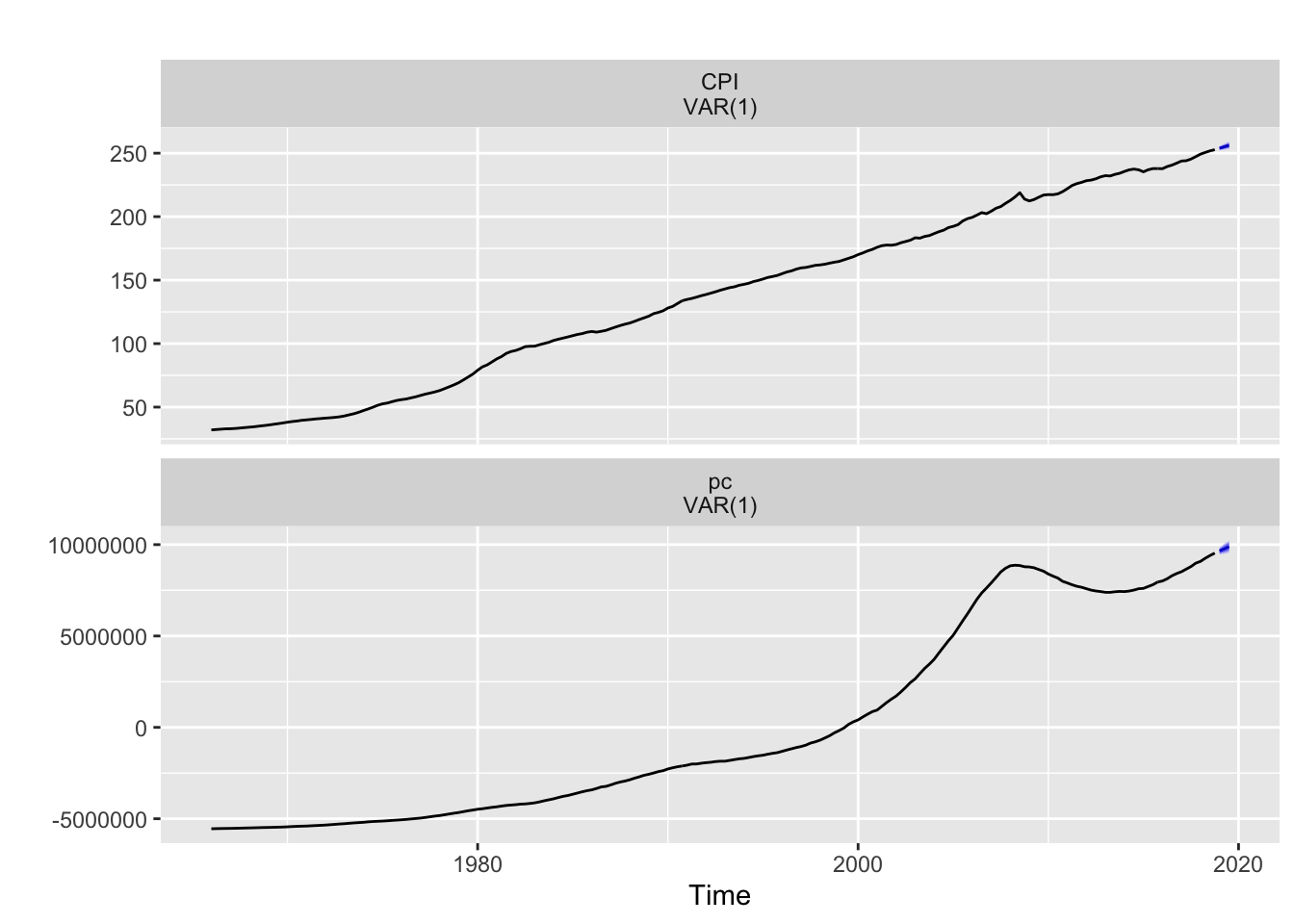
fvar2$forecast$CPI## Point Forecast Lo 80 Hi 80 Lo 95 Hi 95
## 2019 Q1 253.8980 252.8307 254.9653 252.2657 255.5303
## 2019 Q2 255.0371 253.5255 256.5487 252.7254 257.3489
## 2019 Q3 256.1764 254.3224 258.0304 253.3409 259.0118The Vector Autoregressive model with Principal component suggests that for the first quarter of 2019, the CPI will be 253.8980. The exact meaning of the Principal component is hard to interpret.
Comparing the accuracy PC & ARIMA modelThis is the accuracy of the PC
accuracy(fvar2$forecast$CPI,d=1, D=0)## ME RMSE MAE MPE MAPE MASE ACF1
## Training set -0.0000000000000008418657 0.8268766 0.5443384 -0.0755122 0.5244213 0.4737458 0.3555163This is the accuracy of the ARIMA model.
accuracy(fvar$forecast$CPI,d=1, D=0)## ME RMSE MAE MPE MAPE MASE ACF1
## Training set -0.000000000000000676728 0.77214 0.4828257 -0.05978604 0.4327868 0.4202104 0.01620901Comparing the accuracy model, one can see that the Principal Component’s RMSE is lower than “auto.arima”’s RMSE model. But the difference is meager 0.054. Thus, it’s preferable to use the model with the PC component.